This section is dealing with specific types of analysis performed by MDANSE. If you are not sure where these fit into the general workflow of data analysis, please read MDANSE Workflow.
Analysis: Dynamics
This section contains background theory for following plugins:
Density of States
MDANSE calculates the power spectrum of the velocity correlation function (see the section on Velocity Correlation Function), which includes the Fourier transform of the cartesian products of the velocity correlation function such as the Fourier transform of the time correlation between the \(x\) and \(y\) components of the velocity
where \(C_{v_x v_y\alpha\alpha}\left( \omega \right)\) is the Fourier transform of the of the velocity correlation function average over atoms of type \(\alpha\), and \(v_{x,j}\) and \(v_{y,j}\) are the \(x\) and \(y\) components of the velocity of atom \(j\).
The Fourier transform of the mass-weighted velocity autocorrelation function (average of the diagonal terms of the mass-weighted velocity correlation function) for a harmonic system is the vibrational DOS
where \(W_{\alpha}\) is the weighting factor of atom type \(\alpha\). Since the DOS is computed from the unnormalized velocity autocorrelation function, the DOS at \(\omega=0\) gives an approximate value for the diffusion constant (see Eq. (83)) when an equal weighting scheme is used. The DOS can be smoothed by, for example, a Gaussian window applied in the time domain [Ref10] (see the section Time Series); the diffusion constant obtained from this DOS is biased due to the spectral smoothing procedure.
MDANSE computes the density of states starting from atomic velocities. In the case that velocities are not available, the velocities will be computed by numerical differentiation of the coordinate trajectories correcting first for possible jumps due to periodic boundary conditions.
The DOS is also related to the DISF, since for isotropic systems
so that DOS result relevant to neutron experiment measuring the vibrational (or phonon)
density of states can be calculated by using the b_incoherent weight setting.
Mean Square Displacement
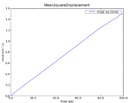
Fig. 6 MSD calculated for a 100 ps MD simulation of 256 water molecules using NPT condition at 1 bar and 300 K.
Molecules in liquids and gases do not stay in the same place but move constantly. This process is called diffusion and it happens quite naturally in fluids at equilibrium. During this process, the motion of an individual molecule does not follow a simple path. As it travels, the molecule undergoes some collisions with other molecules which prevent it from following a straight line. If the path is examined in close detail, it will be seen to be a good approximation to a random walk. Mathematically, a random walk is a series of steps where each step is taken in a completely random direction from the one before. This kind of path was famously analysed by Albert Einstein in a study of Brownian motion. He showed that the Mean-Square Displacement (MSD) of a particle following a random walk is proportional to the time elapsed. The Fig. 6 shows an example of an MSD analysis performed on a water box of 768 water molecules. To get the diffusion coefficient out of this plot, the slope of the linear part of the plot should be calculated.
By defining \(\mathbf{d}_{j}(t) = \mathbf{r}_{j}(t) - \mathbf{r}_{j}(0)\) the MSD of particle \(j\) can be written as
where \(\mathbf{r}_{j}(0)\) and \(\mathbf{r}_{j}(t)\) are the position of particle \(j\) at times \(0\) and \(t\) and \(d_{j}( t ) = \vert \mathbf{d}_{j}(t) \vert\). One can introduce an MSD with respect to a given axis \(\mathbf{n}\)
where \(\hat{\mathbf{n}}\) is a unit vector along \(\mathbf{n}\).
The calculation of MSD is the standard way to obtain diffusion coefficients from MD simulations. Assuming Einstein-diffusion in the long time limit one has for isotropic systems
There exists also a well-known relation between the MSD and the velocity autocorrelation function. One can show (see e.g. [Ref11]) that
where \(C_{\mathbf{vv}jj}(t)\) is the velocity autocorrelation function of the particle \(j\). Using now the definition of the diffusion coefficient Eq. (58) one obtains the relations
Computationally, the MSD is calculated by calculating the position autocorrelation since from Eq. (56)
where the last part on the right side Eq. (61) is the position autocorrelation of the particle \(j\).
Position Correlation Function
The position correlation function (PCF) is similar to the velocity correlation function in Velocity Correlation Function. In MDANSE the PCF is calculated relative to the atoms average position over the entire trajectory. The position autocorrelation function (average of the diagonal terms of the PCF) of atom type \(\alpha\) is
where
so that the origin dependence of the position autocorrelation function is removed.
Position Power Spectrum
The position power spectrum is similar to the density of states calculation in Density of States but is instead a Fourier transform of the PCF. The average of the diagonal terms of the PPS is
and is related to the vibrational DOS via the expresssion
Reorientational Time Correlation Function
Reorientational Time-Correlation Function (RTCF) describes the change in orientation of a specific direction axis within a molecule. This axis is usually defined as a vector between two specific atoms in the molecule, or between one atom and the molecule’s centre of mass.
Reorientational time-correlation functions can be Legendre polynomials of different order. At the moment, this analysis will calculate all the orders up the maximum Legendre polynomial order specified as one of the input parameters.
Angle at time \(t\) is calculated as the following:
The general result is \(C_{l}(t) = \langle P_{l}[\cos(\phi(t))] \rangle\), where \(P_{l}[x]\) is the Legendre polynomial of the order \(l\).
Root Mean Square Deviation
The root mean-square deviation (RMSD) is perhaps the most popular estimator of structural similarity. It quantifies differences between two structures by measuring the root mean-square of atomic position differences, revealing insights into their structural dissimilarities. It is a numerical measure of the difference between two structures. Typically, RMSD is used to quantify the structural evolution of the system during the simulation. It can be used to verify if the simulated system has reached equilibrium or, conversely, if major structural changes occurred during the simulation. The RMSD for the atom of type \(\alpha\) can be defined as
where \(\mathbf{r}_{j}(t)\) and \(\mathbf{r}_{j}(t_{\mathrm{ref}})\) are respectively the position of atom \(j\) at time \(t\) and \(t_{\mathrm{ref}}\) where \(t_{\mathrm{ref}}\) is a reference time usually chosen as the zeroth time of the simulation. As with other analysis jobs in MDANSE, the RMSD results can be grouped. The grouping is slightly different to all other analysis calculations; see Root Mean Square Deviation for more details.
Root Mean Square Fluctuation
The root mean square fluctuation (RMSF) measures the average magnitude of deviations or fluctuations in atomic positions from their mean positions during a simulation. RMSF analysis is valuable for understanding the flexibility and stability of different components of the system, providing insights into regions where atoms or groups of atoms exhibit significant fluctuations. This information can be crucial for studying the dynamic behavior of biomolecules, protein-ligand interactions, or any molecular systems subject to temporal variations. Unlike other job types in MDANSE, the RMSF is only calculated for each atom
so that \(\mathrm{RMSF}_{j}\) is the RMSF for the atom \(j\). As with other analysis jobs in MDANSE, the RMSF results can be grouped. This grouping is slightly different to all other analysis calculations; see Root Mean Square Fluctuation for more details.
Van Hove Function
The van Hove function describes the probability of finding a particle \(k\) at time \(t\) with a displacement of \(\mathbf{r}\) from a particle \(j\) at a time \(0\). In MDANSE the van Hove function is written as a weighted sum of partial terms which are divided by the density
The van Hove function is related to the intermediate scattering function via a Fourier transform and the dynamic structure factor via a double Fourier transform
and can be split into distinct and self parts where
At \(t = 0\) distinct-part of the van Hove function reduces to the pair distribution function while the self-part of the van Hove function becomes a delta function
where \(g_{\alpha\beta}(\mathbf{r})\) is the partial pair distribution function. For liquid or gaseous systems,
where in the thermodynamic limit \(N \rightarrow \infty\).
Velocity Correlation Function
The Velocity Correlation Function (VCF) is a property describing the dynamics of a molecular system. It reveals the underlying nature of the forces acting on the system. For a harmonic system, the Fourier transform of the average of the diagonal components, the velocity autocorrelation function (VACF), is related to the vibrational density of states.
In a molecular system that would be made of non-interacting particles, the velocities would be constant and the VACF would have a constant value. Now, if we think about a system with small interactions such as in a gas-phase, the magnitude and direction of the velocity of a particle will change gradually over time due to its collision with the other particles of the molecular system. In such a system, the VACF will be represented by a decaying exponential.
In the case of solid phase, the interactions are much stronger and, as a results, the atoms are bound to a given position from which they will move backwards and forwards oscillating between positive and negative values of their velocity. The oscillations will not be of equal magnitude however, but will decay in time, because there are still perturbative forces acting on the atoms to disrupt the perfection of their oscillatory motion. So, in that case the VACF will look like a damped harmonic motion.
Finally, in the case of liquid phase, the atoms have more freedom than in solid phase and because of the diffusion process, the oscillatory motion seen in solid phase will be cancelled quite rapidly depending on the density of the system. So, the VACF will just have one very damped oscillation before decaying to zero. This decaying time can be considered as the average time for a collision between two atoms to occur before they diffuse away.
The VCF of atom \(j\) in an atomic or molecular system is defined as between the \(x\) and \(y\) components of the velocity is defined as
while the VACF of atom \(j\) in an atomic or molecular system is defined as
In some cases, e.g. for non-isotropic systems, it is useful to define VACF along a given axis,
where the vector \(\hat{\mathbf{n}}\) is a unit vector defining a space-fixed axis. The VACF of the particles in a many-body system can be related to the incoherent dynamic structure factor by the relation
where \(\hat{\mathbf{q}}\) is the unit vector in the direction of \(\mathbf{q}\). Here the total density of states is a weighted sum of the Fourier transform of the projected VACF
Provided the VACF decays to zero at long time, the function may be integrated mathematically to calculate the diffusion coefficient \(D\), as in:
This is a special case of a more general relationship between the VACF and the mean square displacement, and belongs to a class of properties known as the Green-Kubo relations, which relate correlation functions to so-called transport coefficients.