This section is dealing with specific types of analysis performed by MDANSE. If you are not sure where these fit into the general workflow of data analysis, please read MDANSE Workflow.
Analysis: Dynamics
This section contains background theory for following plugins:
Density of States
MDANSE calculates the power spectrum of the VACF (see the section on Velocity Autocorrelation Function), which in case of the mass-weighted VACF defines the phonon discrete DOS as
where \(C_{\mathbf{vv}\alpha\alpha}\left( \omega \right)\) is the Fourier transform of the velocity autocorrelation function average over atoms of type \(\alpha\), \(W_{\alpha}\) is the weighting factor of atom type \(\alpha\). The DOS can be computed either for the isotropic case or with respect to a user-defined axis.
Since the DOS is computed from the unnormalized VACF, the DOS at \(\omega=0\) gives an approximate value for the diffusion constant (see Eq. (75)) when an equal weighting scheme is used. The DOS can be smoothed by, for example, a Gaussian window applied in the time domain [Ref10] (see the section Time Series); the diffusion constant obtained from this DOS is biased due to the spectral smoothing procedure since the VACF is weighted by this window Gaussian function.
MDANSE computes the density of states starting from atomic velocities. In the case that velocities are not available, the velocities will be computed by numerical differentiation of the coordinate trajectories correcting first for possible jumps due to periodic boundary conditions.
The DOS is also related to the DISF, since for isotropic systems
so that DOS result relevant to neturon experiment measuring the vibrational (or phonon)
density of states can be calculated by using the b_incoherent weight setting.
Mean Square Displacement
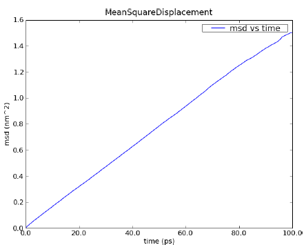
Fig. 6 MSD calculated for a 100 ps MD simulation of 256 water molecules using NPT condition at 1 bar and 300 K.
Molecules in liquids and gases do not stay in the same place but move constantly. This process is called diffusion and it happens quite naturally in fluids at equilibrium. During this process, the motion of an individual molecule does not follow a simple path. As it travels, the molecule undergoes some collisions with other molecules which prevent it from following a straight line. If the path is examined in close detail, it will be seen to be a good approximation to a random walk. Mathematically, a random walk is a series of steps where each step is taken in a completely random direction from the one before. This kind of path was famously analysed by Albert Einstein in a study of Brownian motion. He showed that the Mean-Square Displacement (MSD) of a particle following a random walk is proportional to the time elapsed. The Fig. 6 shows an example of an MSD analysis performed on a water box of 768 water molecules. To get the diffusion coefficient out of this plot, the slope of the linear part of the plot should be calculated.
By defining \(\mathbf{d}_{j}(t) = \mathbf{r}_{j}(t) - \mathbf{r}_{j}(0)\) the MSD of particle \(j\) can be written as
where \(\mathbf{r}_{j}(0)\) and \(\mathbf{r}_{j}(t)\) are the position of particle \(j\) at times \(0\) and \(t\) and \(d_{j}( t ) = \vert \mathbf{d}_{j}(t) \vert\). One can introduce an MSD with respect to a given axis \(\mathbf{n}\)
where \(\hat{\mathbf{n}}\) is a unit vector along \(\mathbf{n}\).
The calculation of MSD is the standard way to obtain diffusion coefficients from MD simulations. Assuming Einstein-diffusion in the long time limit one has for isotropic systems
There exists also a well-known relation between the MSD and the velocity autocorrelation function. One can show (see e.g. [Ref11]) that
where \(C_{\mathbf{vv}jj}(t)\) is the velocity autocorrelation function of the particle \(j\). Using now the definition of the diffusion coefficient Eq. (54) one obtains the relations
Computationally, the MSD is calculated by calculating the position autocorrelation since from Eq. (52)
where the last part on the right side Eq. (57) is the position autocorrelation of the particle \(j\).
Order Parameter
Note
This job is currently not available. The documentation here is out-dated and only left here for referencing purposes.
Adequate and accurate cross comparison of the NMR and MD simulation data is of crucial importance in versatile studies conformational dynamics of proteins. NMR relaxation spectroscopy has proven to be a unique approach for a site-specific investigation of both global tumbling and internal motions of proteins. The molecular motions modulate the magnetic interactions between the nuclear spins and lead for each nuclear spin to a relaxation behaviour which reflects its environment. Since its first applications to the study of protein dynamics, a wide variety of experiments has been proposed to investigate backbone as well as side chain dynamics. Among them, the heteronuclear relaxation measurement of amide backbone 15N nuclei is one of the most widespread techniques. The relationship between microscopic motions and measured spin relaxation rates is given by Redfield’s theory [Ref13]. Under the hypothesis that 15N relaxation occurs through dipole-dipole interactions with the directly bonded 1H atom and chemical shift anisotropy (CSA), and assuming that the tensor describing the CSA is axially symmetric with its axis parallel to the N-H bond, the relaxation rates of the 15N nuclei are determined by a time correlation function,
which describes the dynamics of a unit vector \(\mu_{i}(t)\) pointing along the 15N-1H bond of the residue \(i\) in the laboratory frame. Here \(P_{2}(x)\) is the second order Legendre polynomial. The Redfield theory shows that relaxation measurements probe the relaxation dynamics of a selected nuclear spin only at a few frequencies. Moreover, only a limited number of independent observables are accessible. Hence, to relate relaxation data to protein dynamics one has to postulate either a dynamical model for molecular motions or a functional form for \(C_{ii}(t)\), yet depending on a limited number of adjustable parameters. Usually, the tumbling motion of proteins in solution is assumed isotropic and uncorrelated with the internal motions, such that:
where \(C^{\mathrm{G}}(t)\) and \(C_{\mathit{ii}}^{\mathrm{I}}(t)\) denote the global and the internal time correlation function, respectively. Within the so-called model free approach [Ref14], [Ref15] the internal correlation function is modelled by an exponential,
Here the asymptotic value
is the so-called generalized order parameter, which indicates the degree of spatial restriction of the internal motions of a bond vector, while the characteristic time \(\tau_{\mathrm{eff},i}\) is an effective correlation time, setting the time scale of the internal relaxation processes. \(S_{i}^{2}\) can adopt values ranging from \(0\) (completely disordered) to \(1\) (fully ordered). So, \(S_{i}^{2}\) is the appropriate indicator of protein backbone motions in computationally feasible timescales as it describes the spatial aspects of the reorientational motion of N-H peptidic bonds vector.
When performing order parameter analysis, MDANSE computes for each residue \(i\) both \(C_{\mathit{ii}}(t)\) and \(S_{i}^{2}\). It also computes a correlation function averaged over all the selected bonds defined as:
where \(N_{\mathrm{bonds}}\) is the number of selected bonds for the analysis.
Position Autocorrelation Function
The position autocorrelation function (PACF) is similar to the velocity autocorrelation function in Velocity Autocorrelation Function. In MDANSE the PACF is calculated relative to the atoms average position over the entire trajectory. The PACF of atom type \(\alpha\) is
where
so that the origin dependence of the PACF function is removed.
Reorientational Time Correlation Function
Reorientational Time-Correlation Function (RTCF) describes the change in orientation of a specific direction axis within a molecule. This axis is usually defined as a vector between two specific atoms in the molecule, or between one atom and the molecule’s centre of mass.
Reorientational time-correlation functions can be Legendre polynomials of different order. At the moment, this analysis will calculate all the orders up the maximum Legendre polynomial order specified as one of the input parameters.
Angle at time \(t\) is calculated as the following:
The general result is \(C_{l}(t) = \langle P_{l}[\cos(\phi(t))] \rangle\), where \(P_{l}[x]\) is the Legendre polynomial of the order \(l\).
Root Mean Square Deviation
The root mean-square deviation (RMSD) is perhaps the most popular estimator of structural similarity. It quantifies differences between two structures by measuring the root mean-square of atomic position differences, revealing insights into their structural dissimilarities. It is a numerical measure of the difference between two structures. For the RMSD of the atom of type \(\alpha\) can be defined as
where \(\mathbf{r}_{j}(t)\) and \(\mathbf{r}_{j}(t_{\mathrm{ref}})\) are respectively the position of atom \(j\) at time \(t\) and \(t_{\mathrm{ref}}\) where \(t_{\mathrm{ref}}\) is a reference time usually chosen as the zeroth time of the simulation. Typically, RMSD is used to quantify the structural evolution of the system during the simulation. It can provide precious information about the system especially if it reached equilibrium or conversely if major structural changes occurred during the simulation.
Root Mean Square Fluctuation
Root mean square fluctuation (RMSF) assesses how the positions of atoms or molecules within a system fluctuate over time. Specifically, RMSF measures the average magnitude of deviations or fluctuations in atomic positions from their mean positions during a simulation. RMSF analysis is valuable for understanding the flexibility and stability of molecules within a simulation, providing insights into regions where atoms or groups of atoms exhibit significant fluctuations. This information can be crucial for studying the dynamic behavior of biomolecules, protein-ligand interactions, or any molecular system subject to temporal variations.
Van Hove Function
The van Hove function describes the probability of finding a particle \(k\) at time \(t\) with a displacement of \(\mathbf{r}\) from a particle \(j\) at a time \(0\). In MDANSE the van Hove function is written as a weighted sum of partial terms which are divided by the density
The van Hove function is related to the intermediate scattering function via a Fourier transform and the dynamic structure factor via a double Fourier transform
and can be split into distinct and self parts where
At \(t = 0\) distinct-part of the van Hove function reduces to the pair distribution function while the self-part of the van Hove function becomes a delta function
where \(g_{\alpha\beta}(\mathbf{r})\) is the partial pair distribution function. For liquid or gaseous systems,
where in the thermodynamic limit \(N \rightarrow \infty\).
Velocity Autocorrelation Function
The Velocity AutoCorrelation Function (VACF) is a property describing the dynamics of a molecular system. It reveals the underlying nature of the forces acting on the system. Its Fourier Transform gives the cartesian density of states for a set of atoms.
In a molecular system that would be made of non-interacting particles, the velocities would be constant and the VACF would have a constant value. Now, if we think about a system with small interactions such as in a gas-phase, the magnitude and direction of the velocity of a particle will change gradually over time due to its collision with the other particles of the molecular system. In such a system, the VACF will be represented by a decaying exponential.
In the case of solid phase, the interactions are much stronger and, as a results, the atoms are bound to a given position from which they will move backwards and forwards oscillating between positive and negative values of their velocity. The oscillations will not be of equal magnitude however, but will decay in time, because there are still perturbative forces acting on the atoms to disrupt the perfection of their oscillatory motion. So, in that case the VACF will look like a damped harmonic motion.
Finally, in the case of liquid phase, the atoms have more freedom than in solid phase and because of the diffusion process, the oscillatory motion seen in solid phase will be cancelled quite rapidly depending on the density of the system. So, the VACF will just have one very damped oscillation before decaying to zero. This decaying time can be considered as the average time for a collision between two atoms to occur before they diffuse away.
Mathematically, the VACF of atom \(j\) in an atomic or molecular system is usually defined as
In some cases, e.g. for non-isotropic systems, it is useful to define VACF along a given axis,
where the vector \(\hat{\mathbf{n}}\) is a unit vector defining a space-fixed axis. The VACF of the particles in a many-body system can be related to the incoherent dynamic structure factor by the relation
where \(\hat{\mathbf{q}}\) is the unit vector in the direction of \(\mathbf{q}\). Here the total density of states is a weighted sum of the Fourier transform of the projected VACF
Provided the VACF decays to zero at long time, the function may be integrated mathematically to calculate the diffusion coefficient \(D\), as in:
This is a special case of a more general relationship between the VACF and the mean square displacement, and belongs to a class of properties known as the Green-Kubo relations, which relate correlation functions to so-called transport coefficients.