Obtaining Converged Results
In MD, a large number of settings must be chosen correctly to ensure that high quality results are obtained. Some of these include the size of the MD box, the time step and the simulation length. The choice of these settings also depends on the type of intended analysis; for example, the dynamic coherent structure factor is much more difficult to converge when compared to the dynamics incoherent structure factor. In this section we will show how the calculation results change with different MD settings for a simple liquid argon system.
Simulation Box Size
Pair Distribution Function
Here we run a liquid argon trajectory with four different simulation box sizes: 1.146, 2.292, 4.584 and 9.168 nm. The same atom density, temperature, time step and simulation length are used for all cases. We calculate the pair distribution function for all trajectories.
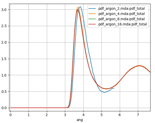
Fig. 7 PDF calculated for a 120 ps MD simulation of liquid argon with a number of different MD box sizes. Blue, orange, green and red plots correspond to MD box sizes of 1.146, 2.292, 4.584 and 9.168 nm respectively.
In Fig. 7 we show the results for the PDF plotted to half the box size. Our smallest box size 1.146 nm (blue in Fig. 7) is small enough for the periodic image of the argon atoms to have a significant effect on itself. Compared to our largest system size, the first peak is shifted to a slightly longer distance, is too high and too broad.
Simulation Length
Dynamic Coherent Structure Factor
For analysis types which calculate a correlation function, a balance between the length of your correlation function and the number of configurations that you average over for each time step must be reached. Here we run dynamic coherent structure factor calculations using the liquid argon trajectory with the 4.584 nm box size, ideal instrument resolution and two different correlation frames settings.
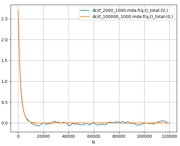
Fig. 8 The coherent intermediate scattering function calculated for 120 ps from a 240 ps and 12 ns MD simulation of liquid argon plotted in blue and orange respectively.
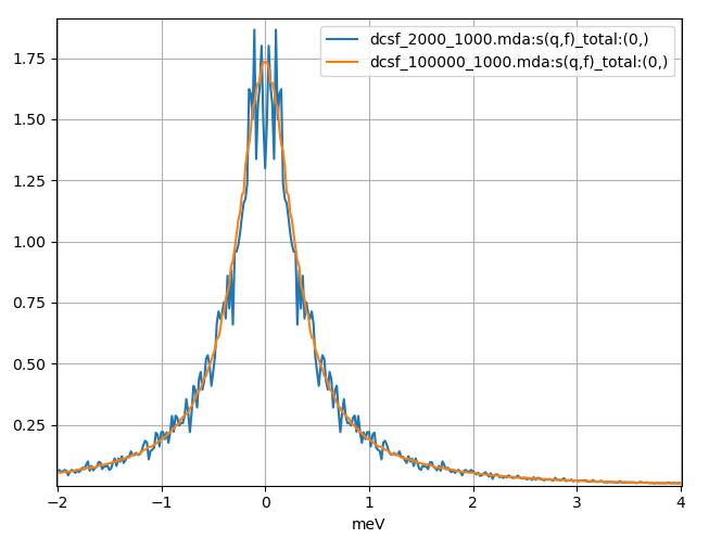
Fig. 9 The dynamic coherent structure factor calculated from a Fourier transform of the above coherent intermediate scattering functions using a 240 ps and 12 ns MD simulation of liquid argon plotted in blue and orange respectively.
In the first calculation (blue in Fig. 8 and Fig. 9), we use a correlation frames setting of (0, 2000, 1, 1000). The first and last frames will be 0 and 2000 and the number of time steps of the correlation function will be 1000. This will mean that for this calculation each time step of the correlation function will be averaged over 1001 = 2000 – 1000 + 1 configurations. For the blue plot in Fig. 8 we can see \(F(q, t)\) oscillate around zero; after Fourier transforming we obtain a noisy \(S(q, f)\) which is especially poor around zero energy.
In the second calculation (orange in Fig. 8 and Fig. 9), we use a correlation frames setting of (0, 100000, 1, 1000). It means that each time step of the correlation function will be averaged over 99001 = 100000 – 1000 + 1 configurations, but will still be the same length as the first calculation. Visually, we can see that \(F(q, t)\) decay and stay closer to zero, and after Fourier transforming we obtain a much smoother \(S(q, f)\). There is still some noise; perhaps an even longer trajectory would be required. Clearly for dynamic coherent structure factor calculations, to obtain high quality results longer trajectories are needed so that a larger number of configurations are used per time step of the correlation function.
In both calculations the number of correlation function time steps was set to 1000, which corresponds to a time of 120 ps. From the \(F(q, t)\), we can see that this is sufficiently long to ensure that the correlation function decays to zero. We can see that it does not change significantly beyond 30 ps or so. For other calculations or systems this might not be the case and a more careful choice for the correlation frames may be required.
Dynamic Incoherent Structure Factor
Here we run the dynamic incoherent structure factor calculations using the same liquid argon system and correlation frames settings as in the dynamic coherent structure factor calculations above.
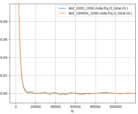
Fig. 10 The incoherent intermediate scattering function calculated for 120 ps from a 240 ps and 12 ns MD simulation of liquid argon plotted in blue and orange respectively.
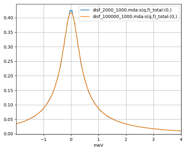
Fig. 11 The dynamic incoherent structure factor calculated from a Fourier transform of the above incoherent intermediate scattering functions using a 240 ps and 12 ns MD simulation of liquid argon plotted in blue and orange respectively.
In contrast to the coherent calculations, there are only minor differences between calculations with the (0, 2000, 1, 1000) and (0, 100000, 1, 1000) correlation frames settings, results shown in blue and orange in Fig. 10 and Fig. 11 respectively. We can see that the incoherent calculation requires a much smaller number of configurations per time step to approach convergence.
Static Structure Factor
Unlike the previous two calculations, the static structure factor does not require the calculations of a correlation function. The quality of your results will depend on the length of your trajectory (among a number of other things) but obviously there will not be a correlation frames setting to specify.
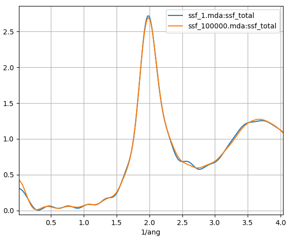
Fig. 12 The static structure factor using a single frame of an MD simulation and a 12 ns MD simulation of liquid argon plotted in blue and orange respectively.
In Fig. 12 we plot the static structure factor calculated from a single frame of an MD simulation and a 12 ns MD simulation. We can see that even when we use a single frame, the SSF is quite close to the results from the 12 ns MD simulation. This occurs since converged results can be obtained for large system sizes or long trajectories. The argon trajectory used contain a total of 2048 atoms which appears to be sufficient to obtain enough statistics for good static structure factor results, so that only a short MD simulation would be required.
Simulation Time Step
Dynamic Incoherent Structure Factor
The DISF (also the DCSF) calculation probes the dynamics of the MD trajectory at different time scales. For example, smaller values of \(q\) correspond to larger time scales while larger values of \(q\) correspond to smaller time scales. To obtain accurate DISF results we therefore need smaller time steps for the larger values of \(q\).
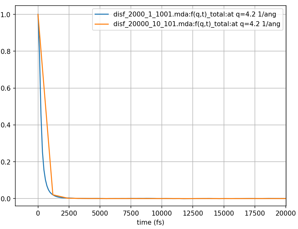
Fig. 13 The incoherent intermediate scattering function calculated for 120 ps from the same MD simulation of liquid argon but with positions sampled every 0.12 and 1.2 ps shown in blue and orange respectively.
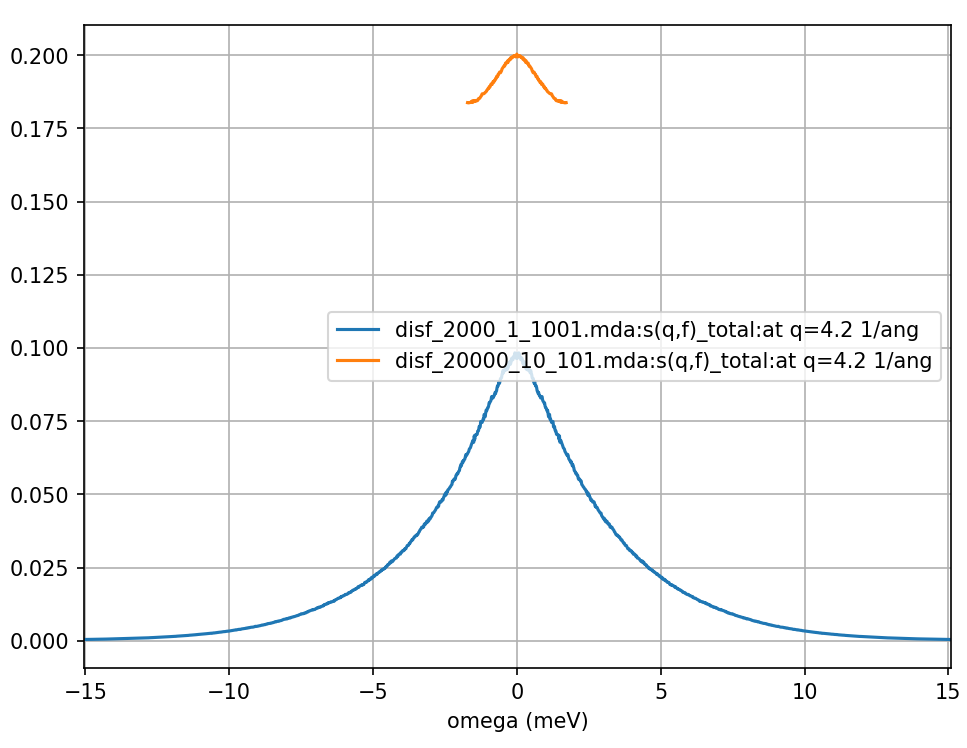
Fig. 14 The dynamic incoherent structure factor calculated from a Fourier transform of the above incoherent intermediate scattering function calculated for 120 ps from the same MD simulation of liquid argon but with positions sampled every 0.12 and 1.2 ps shown in blue and orange respectively.
Here we run DISF calculations with a correlation frames setting of (0, 2000, 1, 1001)
and another with a correlation frames setting of (0, 20000, 10, 101) and set \(q\) to 42 nm-1. The
MD simulation was sampled every 120 fs, so by using a in step of setting
of 10 we are effectively sampling the trajectory every 1.2 ps. For
each frame of the correlation function, the first calculation averages
over 1000 frames while the second averages over 1900 frames. The total
time of the DISF of both calculations will be the same.
As you can see from the Fig. 13 for this larger value of \(q\) the intermediate scattering function decays quickly. We can see that the second calculation (orange in Fig. 13 and Fig. 14) time steps were too long and did not sufficiently sample the intermediate scattering function which had already decayed to zero by the second time step. Looking at Fig. 14 we can see how poor the sampling of the intermediate scattering function was. The resulting DISF (orange curve in Fig. 14) is severely overestimated, does not provide the higher frequency results, and does not follow the same qualitative behaviour as the first calculation (blue curve).
Density of States
The density of states (DOS) is calculated by taking a Fourier transform of the velocity autocorrelation function (VACF). In MDANSE, velocity information from your MD data files can be saved into the MDANSE trajectory file and used in any subsequent analysis calculation. In some cases, you may not have saved the velocity data or you may want to recalculate the velocities from atom positions. In the DOS job you have the option to calculate velocities using numerical derivatives of the atomic positions. The accuracy of these velocities will be highly dependent on the time step of the trajectory.
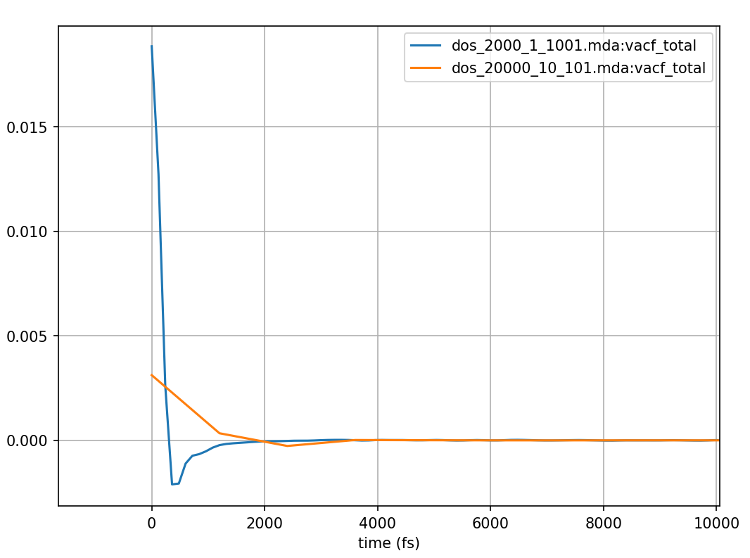
Fig. 15 Velocity autocorrelation function using velocities determined by numerical derivatives of atomic positions from the same MD simulation of liquid argon, but with positions sampled every 0.12 and 1.2 ps shown in blue and orange respectively.
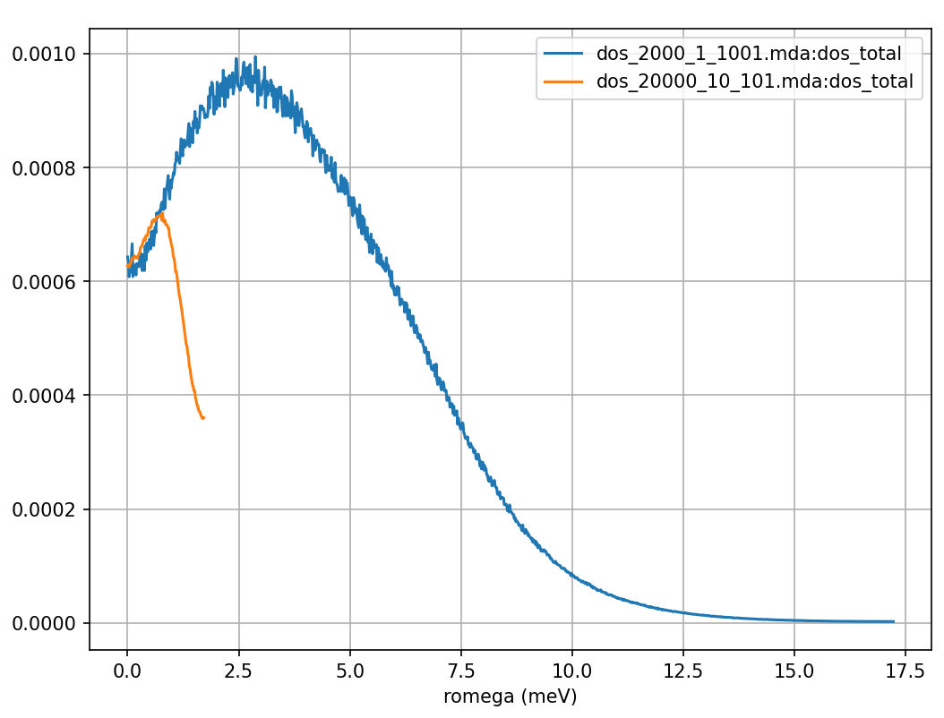
Fig. 16 The density of states calculated from a Fourier transform of the above velocity autocorrelation function calculated from the same MD simulation of liquid argon, but with positions sampled every 0.12 and 1.2 ps shown in blue and orange respectively.
Here we run DOS calculations with a correlation frames setting of (0, 2000, 1, 1001)
and another with a correlation frames setting of (0, 20000, 10, 101). We use
an interpolation order setting of 3 so that velocities will be determined
by a numerical derivative of the atomic positions. Fig. 15
shows that the numerical derivative for the calculation which used the
in step of setting of 10 (orange curves in Fig. 15 and Fig. 16),
had produced a severely underestimated VACF value at \(t=0\). Additionally, the longer time step means that it misses the
trough seen in the blue curve of Fig. 15 between 0
and 2000 fs. The resulting DOS (orange curve in Fig. 16) does not provide the higher frequency
results, has a peak at an incorrect position, and falls off towards zero far too early.
Q Vector Sampling
A note on crystals
If you are simulating a crystal (i.e. a highly ordered, anisotropic material), you will be interested in calculating the observables such as the \(S(\mathbf{q},\omega)\) at specific points in reciprocal space. You will most likely pick a q-vector generator such as DispersionLatticeQVectors, which will generate a single lattice vector per calculated data point. The concept of convergence in respect to q-vector sampling will not apply in this situation.
Isotropic systems
For isotropic, disordered systems, the calculation results will be averaged over vectors with similar \(\vert \mathbf{q} \vert = q\) and output as a function of \(q\). Spherical averaging is most commonly applied, as many systems can be assumed to be fully isotropic. SphericalLatticeQVectors is normally used for calculating the quasielastic neutron scattering results in isotropic systems.
Generating the vectors on a sphere is equivalent to assuming that all the possible scattering geometries are possible, or rotating the simulated system to calculate the scattering results for different orientations of the system. This allows the code to approximate the correct scattering experiment results which would otherwise require a significantly larger simulation. A physical sample in a real-life experiment typically contains in the order of \(10^{23}\) atoms (the Avogadro number), while many MD trajectories contain less than \(10^6\) atoms. Therefore, an actual experiment will sample many more configurations of atoms than it is possible to sample in a single MD simulation. Performing the calculation on multiple Q vectors maximises the information that can be extracted from an MD trajectory. The computational effort of the calculation increases linearly with every additional vector for which the calculation is performed.
Random vector generation
For 1D, 2D and 3D averaging (which could be relevant to calculations on layered, nematic and completely disordered systems, respectively), there exist three vector generators which apply the same approach in different numbers of dimensions:
Each of these will generate vectors randomly within “shells”, following a normal distribution of \(q\) around the specified mean value for each shell. The spatial distribution is constrained to a single line for the linear generator, while for the other two it will be uniform in angles on a circle and a sphere, respectively.
You will most likely need the lattice versions of these generators, which follow the same approach, but apply additional processing steps afterwards.
Lattice vector generators
Once the random vector distribution has been created, the lattice vector generators round the hkl coordinates of all the vectors to the nearest integer values. This will result in some of the vectors arriving at values of \(q\) outside of the specified range, which will then be discarded from the total population. From the remaining vectors, it is likely that multiple randomly generated vectors will end up at the same HKL coordinates after rounding. The number of random vectors rounded to a specific HKL value becomes the weight of that vector in the calculation. The actual calculation is then performed only for the unique lattice vectors.
For shells that are small compared to the size of the system’s unit cell, the number of unique vectors will be small (possibly as low as 6 for the smallest shell in a cubic system). For these, the number of vectors can be increased without increasing the total calculation time, resulting in the relative vector weights converging to equal values. However, for wider shells including vectors with different values of \(q\), the weights will also scale the contributions of vectors to the results based on the difference between the nominal value of \(q\) for the shell and actual values of \(q\) for specific vectors.
For large vector shells which contain many unique vectors, increasing the number of vectors used for sampling will add new lattice vectors to the calculation, increasing the total time needed to complete the calculation.
Convergence of vector sampling
Currently, there is no single answer as to how many vectors need to be used for sampling the reciprocal space. There are two kinds of tests that a user may want to perform to establish if a sufficient number of vectors is being used.
Reproducibility test. The same calculation is repeated several times using different random seeds. The deviation of the calculated results can be used as an estimate of the uncertainty of the results.
Convergence test. The same calculation is repeated with increasing number of vectors used for sampling. The difference between the consecutive runs will keep decreasing.
In both cases, it makes sense to use the measurement uncertainty of the experimental data used as reference to determine the level of accuracy needed in the calculation.